Introduction to Diffusion MRI data

Overview

Teaching: 20 min
Exercises: 5 min

Questions

How is dMRI data represented?

What is diffusion weighting?

Objectives

Representation of diffusion data and associated gradients

Learn about diffusion gradients

Diffusion Weighted Imaging (DWI)

Diffusion MRI is a popular technique to study the brain’s white matter. To do so, sequences sensitive to random, microscropic motion of water protons are applied. The diffusion within biological structures, such as the brain, are often restricted due to barriers (e.g. cell membranes), resulting in a preferred direction of diffusion (anisotropy). A typical diffusion MRI scan will acquire multiple volumes that are sensitive to a particular diffusion direction and result in diffusion-weighted images (DWI). Diffusion that exhibits directionality in the same direction result in an attenuated signal. With further processing (to be discussed later in the lesson), the acquired images can provide measurements which are related to the microscopic changes and estimate white matter trajectories. Images with no diffusion weighting are also acquired as part of the acquisition protocol.

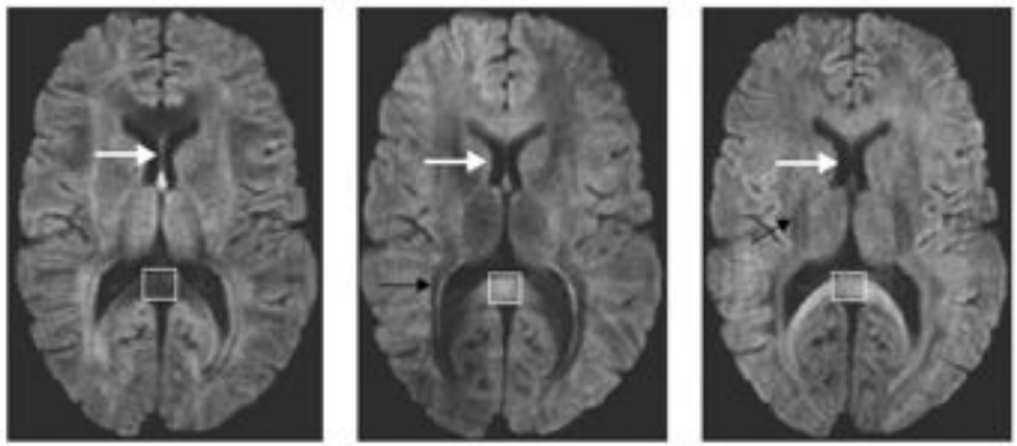
Diffusion along X, Y, and Z directions

b-values & b-vectors

In addition to the acquired diffusion images, two files are collected as part of the diffusion dataset. These files correspond to the gradient amplitude (b-values) and directions (b-vectors) of the diffusion measurement and are named with the extensions .bval and .bvec respectively. The b-value is the diffusion-sensitizing factor, and reflects the timing & strength of the gradients used to acquire the diffusion-weighted images. The b-vector corresponds to the direction of the diffusion sensitivity. Together these two files define the diffusion MRI measurement as a set of gradient directions and corresponding amplitudes.

Dataset

For the rest of this lesson, we will make use of a subset of a publicly available dataset, ds000221, originally hosted at openneuro.org. The dataset is structured according to the Brain Imaging Data Structure (BIDS). Please check the the BIDS-dMRI Setup page to download the dataset.

Below is a tree diagram showing the folder structure of a single MR subject and session within ds000221. This was obtained by using the bash command tree.

tree '../data/ds000221'

../data/ds000221
├── .bidsignore
├── CHANGES
├── dataset_description.json
├── participants.tsv
├── README
├── derivatives/
├── sub-010001/
└── sub-010002/
    ├── ses-01/
    │    ├── anat
    │    │    ├── sub-010002_ses-01_acq-lowres_FLAIR.json
    │    │    ├── sub-010002_ses-01_acq-lowres_FLAIR.nii.gz
    │    │    ├── sub-010002_ses-01_acq-mp2rage_defacemask.nii.gz
    │    │    ├── sub-010002_ses-01_acq-mp2rage_T1map.nii.gz
    │    │    ├── sub-010002_ses-01_acq-mp2rage_T1w.nii.gz
    │    │    ├── sub-010002_ses-01_inv-1_mp2rage.json
    │    │    ├── sub-010002_ses-01_inv-1_mp2rage.nii.gz
    │    │    ├── sub-010002_ses-01_inv-2_mp2rage.json
    │    │    ├── sub-010002_ses-01_inv-2_mp2rage.nii.gz
    │    │    ├── sub-010002_ses-01_T2w.json
    │    │    └── sub-010002_ses-01_T2w.nii.gz
    │    ├── dwi
    │    │    ├── sub-010002_ses-01_dwi.bval
    │    │    │── sub-010002_ses-01_dwi.bvec
    │    │    │── sub-010002_ses-01_dwi.json
    │    │    └── sub-010002_ses-01_dwi.nii.gz
    │    ├── fmap
    │    │    ├── sub-010002_ses-01_acq-GEfmap_run-01_magnitude1.json
    │    │    ├── sub-010002_ses-01_acq-GEfmap_run-01_magnitude1.nii.gz
    │    │    ├── sub-010002_ses-01_acq-GEfmap_run-01_magnitude2.json
    │    │    ├── sub-010002_ses-01_acq-GEfmap_run-01_magnitude2.nii.gz
    │    │    ├── sub-010002_ses-01_acq-GEfmap_run-01_phasediff.json
    │    │    ├── sub-010002_ses-01_acq-GEfmap_run-01_phasediff.nii.gz
    │    │    ├── sub-010002_ses-01_acq-SEfmapBOLDpost_dir-AP_epi.json
    │    │    ├── sub-010002_ses-01_acq-SEfmapBOLDpost_dir-AP_epi.nii.gz
    │    │    ├── sub-010002_ses-01_acq-SEfmapBOLDpost_dir-PA_epi.json
    │    │    ├── sub-010002_ses-01_acq-SEfmapBOLDpost_dir-PA_epi.nii.gz
    │    │    ├── sub-010002_ses-01_acq-sefmapBOLDpre_dir-AP_epi.json
    │    │    ├── sub-010002_ses-01_acq-sefmapBOLDpre_dir-AP_epi.nii.gz
    │    │    ├── sub-010002_ses-01_acq-sefmapBOLDpre_dir-PA_epi.json
    │    │    ├── sub-010002_ses-01_acq-sefmapBOLDpre_dir-PA_epi.nii.gz
    │    │    ├── sub-010002_ses-01_acq-SEfmapBOLDpost_dir-AP_epi.json
    │    │    ├── sub-010002_ses-01_acq-SEfmapBOLDpost_dir-AP_epi.nii.gz
    │    │    ├── sub-010002_ses-01_acq-SEfmapBOLDpost_dir-PA_epi.json
    │    │    ├── sub-010002_ses-01_acq-SEfmapBOLDpost_dir-PA_epi.nii.gz
    │    │    ├── sub-010002_ses-01_acq-SEfmapDWI_dir-AP_epi.json
    │    │    ├── sub-010002_ses-01_acq-SEfmapDWI_dir-AP_epi.nii.gz
    │    │    ├── sub-010002_ses-01_acq-SEfmapDWI_dir-PA_epi.json
    │    │    └── sub-010002_ses-01_acq-SEfmapDWI_dir-PA_epi.nii.gz
    │    └── func
    │    │    ├── sub-010002_ses-01_task-rest_acq-AP_run-01_bold.json
    │    │    └── sub-010002_ses-01_task-rest_acq-AP_run-01_bold.nii.gz
    └── ses-02/

Querying a BIDS Dataset

PyBIDS is a Python package for querying, summarizing and manipulating the BIDS folder structure. We will make use of PyBIDS to query the necessary files.

Let’s first pull the metadata from its associated JSON file using the get_metadata() function for the first run.

from bids.layout import BIDSLayout

?BIDSLayout

layout = BIDSLayout("../data/ds000221", validate=False)

Now that we have a layout object, we can work with a BIDS dataset! Let’s extract the metadata from the dataset.

dwi = layout.get(subject='010006', suffix='dwi', extension='.nii.gz', return_type='file')[0]
layout.get_metadata(dwi)

{'EchoTime': 0.08,
 'EffectiveEchoSpacing': 0.000390001,
 'FlipAngle': 90,
 'ImageType': ['ORIGINAL', 'PRIMARY', 'DIFFUSION', 'NON'],
 'MagneticFieldStrength': 3,
 'Manufacturer': 'Siemens',
 'ManufacturersModelName': 'Verio',
 'MultibandAccelerationFactor': 2,
 'ParallelAcquisitionTechnique': 'GRAPPA',
 'ParallelReductionFactorInPlane': 2,
 'PartialFourier': '7/8',
 'PhaseEncodingDirection': 'j-',
 'RepetitionTime': 7,
 'TotalReadoutTime': 0.04914}

Diffusion Imaging in Python (DIPY)

For this lesson, we will use the DIPY (Diffusion Imaging in Python) package for processing and analysing diffusion MRI.

Why `DIPY`?

Fully free and open source.
Implemented in Python. Easy to understand, and easy to use.
Implementations of many state-of-the art algorithms.
High performance. Many algorithms implemented in Cython.

Defining a measurement: `GradientTable`

DIPY has a built-in function that allows us to read in bval and bvec files named read_bvals_bvecs under the dipy.io.gradients module. Let’s first grab the path to our gradient directions and amplitude files and load them into memory.

bvec = layout.get_bvec(dwi)
bval = layout.get_bval(dwi)

Now that we have the necessary diffusion files, let’s explore the data!

import numpy as np
import nibabel as nib

from mpl_toolkits.mplot3d import Axes3D
import matplotlib.pyplot as plt

data = nib.load(dwi).get_fdata()
data.shape

(128, 128, 88, 67)

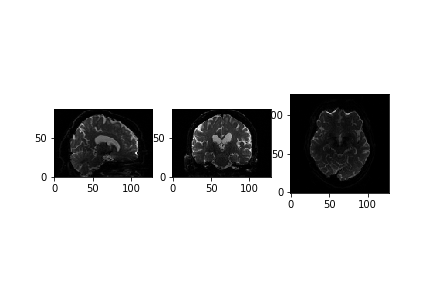
We can see that the data is 4 dimensional. The 4th dimension represents the different diffusion directions we are sensitive to. Next, let’s take a look at a slice.

x_slice = data[58, :, :, 0]
y_slice = data[:, 58, :, 0]
z_slice = data[:, :, 30, 0]

slices = [x_slice, y_slice, z_slice]

fig, axes = plt.subplots(1, len(slices))
for i, _slice in enumerate(slices):
    axes[i].imshow(_slice.T, cmap="gray", origin="lower")

DWI slice

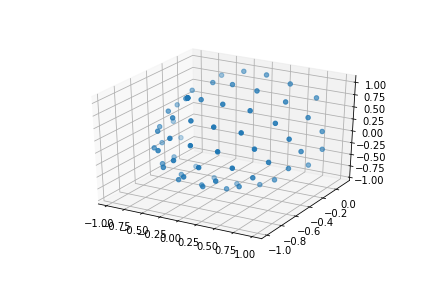
We can also see how the diffusion gradients are represented. This is plotted on a sphere, the further away from the center of the sphere, the stronger the diffusion gradient (increased sensitivity to diffusion).

bvec_txt = np.genfromtxt(bvec)

fig = plt.figure()
ax = fig.add_subplot(111, projection='3d')
ax.scatter(bvec_txt[0], bvec_txt[1], bvec_txt[2])

plt.show()

Diffusion gradient sphere

The files associated with the diffusion gradients need to converted to a GradientTable object to be used with DIPY. A GradientTable object can be implemented using the dipy.core.gradients module. The input to the GradientTable should be our the values for our gradient directions and amplitudes we read in.

from dipy.io.gradients import read_bvals_bvecs
from dipy.core.gradients import gradient_table

gt_bvals, gt_bvecs = read_bvals_bvecs(bval, bvec)
gtab = gradient_table(gt_bvals, gt_bvecs)

We will need this gradient table later on to process our data and generate diffusion tensor images (DTI)!

There is also a built-in function for gradient tables, b0s_mask that can be used to separate diffusion weighted measurements from non-diffusion weighted measurements ($b = 0 s/mm^2$, commonly referred to as the B0 volume or image). We will extract the vector corresponding to diffusion weighted measurements!

gtab.bvecs[~gtab.b0s_mask]

array([[-2.51881e-02, -3.72268e-01,  9.27783e-01],
       [ 9.91276e-01, -1.05773e-01, -7.86433e-02],
       [-1.71007e-01, -5.00324e-01, -8.48783e-01],
       [-3.28334e-01, -8.07475e-01,  4.90083e-01],
       [ 1.59023e-01, -5.08209e-01, -8.46425e-01],
       [ 4.19677e-01, -5.94275e-01,  6.86082e-01],
       [-8.76364e-01, -4.64096e-01,  1.28844e-01],
       [ 1.47409e-01, -8.01322e-02,  9.85824e-01],
       [ 3.50020e-01, -9.29191e-01, -1.18704e-01],
       [ 6.70475e-01,  1.96486e-01,  7.15441e-01],
       [-6.85569e-01,  2.47048e-01,  6.84808e-01],
       [ 3.21619e-01, -8.24329e-01,  4.65879e-01],
       [-8.35634e-01, -5.07463e-01, -2.10233e-01],
       [ 5.08740e-01, -8.43979e-01,  1.69950e-01],
       [-8.03836e-01, -3.83790e-01,  4.54481e-01],
       [-6.82578e-02, -7.53445e-01, -6.53959e-01],
       [-2.07898e-01, -6.27330e-01,  7.50490e-01],
       [ 9.31645e-01, -3.38939e-01,  1.30988e-01],
       [-2.04382e-01, -5.95385e-02,  9.77079e-01],
       [-3.52674e-01, -9.31125e-01, -9.28787e-02],
       [ 5.11906e-01, -7.06485e-02,  8.56132e-01],
       [ 4.84626e-01, -7.73448e-01, -4.08554e-01],
       [-8.71976e-01, -2.40158e-01, -4.26593e-01],
       [-3.53191e-01, -3.41688e-01,  8.70922e-01],
       [-6.89136e-01, -5.16115e-01, -5.08642e-01],
       [ 7.19336e-01, -5.25068e-01, -4.54817e-01],
       [ 1.14176e-01, -6.44483e-01,  7.56046e-01],
       [-5.63224e-01, -7.67654e-01, -3.05754e-01],
       [-5.31237e-01, -1.29342e-02,  8.47125e-01],
       [ 7.99914e-01, -7.30043e-02,  5.95658e-01],
       [-1.43792e-01, -9.64620e-01,  2.20979e-01],
       [ 9.55196e-01, -5.23107e-02,  2.91314e-01],
       [-3.64423e-01,  2.53394e-01,  8.96096e-01],
       [ 6.24566e-01, -6.44762e-01,  4.40680e-01],
       [-3.91818e-01, -7.09411e-01, -5.85845e-01],
       [-5.21993e-01, -5.74810e-01,  6.30172e-01],
       [ 6.56573e-01, -7.41002e-01, -1.40812e-01],
       [-6.68597e-01, -6.60616e-01,  3.41414e-01],
       [ 8.20224e-01, -3.72360e-01,  4.34259e-01],
       [-2.05263e-01, -9.02465e-01, -3.78714e-01],
       [-6.37020e-01, -2.83529e-01,  7.16810e-01],
       [ 1.37944e-01, -9.14231e-01, -3.80990e-01],
       [-9.49691e-01, -1.45434e-01,  2.77373e-01],
       [-7.31922e-03, -9.95911e-01, -9.00386e-02],
       [-8.14263e-01, -4.20783e-02,  5.78969e-01],
       [ 1.87418e-01, -9.63210e-01,  1.92618e-01],
       [ 3.30434e-01,  1.92714e-01,  9.23945e-01],
       [ 8.95093e-01, -2.18266e-01, -3.88805e-01],
       [ 3.11358e-01, -3.49170e-01,  8.83819e-01],
       [-6.86317e-01, -7.27289e-01, -4.54356e-03],
       [ 4.92805e-01, -5.14280e-01, -7.01897e-01],
       [-8.03482e-04, -8.56796e-01,  5.15655e-01],
       [-4.77664e-01, -4.45734e-01, -7.57072e-01],
       [ 7.68954e-01, -6.22151e-01,  1.47095e-01],
       [-1.55099e-02,  2.22329e-01,  9.74848e-01],
       [-9.74410e-01, -2.11297e-01, -7.66740e-02],
       [ 2.56251e-01, -7.33793e-01, -6.29193e-01],
       [ 6.24656e-01, -3.42071e-01,  7.01992e-01],
       [-4.61411e-01, -8.64670e-01,  1.98612e-01],
       [ 8.68547e-01, -4.66754e-01, -1.66634e-01]])

It is also important to know where our diffusion weighting free measurements are as we need them for registration in our preprocessing, (our next notebook). gtab.b0s_mask shows that this is our first volume of our dataset.

gtab.b0s_mask

array([ True, False, False, False, False, False, False, False, False,
       False, False,  True, False, False, False, False, False, False,
       False, False, False, False,  True, False, False, False, False,
       False, False, False, False, False, False,  True, False, False,
       False, False, False, False, False, False, False, False,  True,
       False, False, False, False, False, False, False, False, False,
       False,  True, False, False, False, False, False, False, False,
       False, False, False,  True])

In the next few notebooks, we will talk more about preprocessing the diffusion weighted images, reconstructing the diffusion tensor model, and reconstruction axonal trajectories via tractography.

Exercise 1

Get a list of all diffusion data in NIfTI file format
Solution
dwi_data = layout.get(suffix='dwi', extension='.nii.gz', return_type='file')

Key Points

dMRI data is represented as a 4-dimensional image (x,y,z,diffusion directional sensitivity)

dMRI data is sensitive to a particular direction of diffusion motion. Due to this sensitivity, each volume of the 4D image is sensitive to a particular direction

lesson home

Introduction to dMRI

next episode

Introduction to Diffusion MRI data

Overview

Diffusion Weighted Imaging (DWI)

b-values & b-vectors

Dataset

Querying a BIDS Dataset

Diffusion Imaging in Python (DIPY)

Why `DIPY`?

Defining a measurement: `GradientTable`

Exercise 1

Solution

Key Points

lesson home

next episode

lesson home

Introduction to dMRI

next episode

Introduction to Diffusion MRI data

Overview

Diffusion Weighted Imaging (DWI)

b-values & b-vectors

Dataset

Querying a BIDS Dataset

Diffusion Imaging in Python (DIPY)

Why DIPY?

Defining a measurement: GradientTable

Exercise 1

Solution

Key Points

lesson home

next episode

Why `DIPY`?

Defining a measurement: `GradientTable`